Dynamics of Blade With
Geometrical Nonlinearity
Department
of Nonstationary Vibrations, A.N. Podgorny Institute for Mechanical Engineering
Problems,
1e-mail:
id.breslavsky@gmail.com
2e-mail:
kvavr@kharkov.ua
Abstract:
The compressor blade is described by pre-twisted,
variable thickness, double curvature shallow shell with geometrical
nonlinearity. The R-function method and the Rayleigh- Ritz approach are used
collectively to calculate eigenmodes of linear vibrations.
Nonlinear vibrations of shell are approximated by using these eigenmodes. The
obtained finite degrees-of-freedom system has three internal resonances. The
free nonlinear vibrations are studied by nonlinear modes.
Keywords: shallow
shells, finite degree-of-freedom system, internal resonances, nonlinear normal
modes
*Corresponding author. Tel.: +38 057 3494783; Fax: +38 0572
944635.
1. Introduction
Significant
dynamics loads act on the blades of turbo machine during their operation. Therefore,
blades can perform vibrations with amplitudes commensurable with their
thickness. Such blade deformations are described by geometrical nonlinear
theory. Many efforts have been done to study blade vibrations. Venkatsan,
Nagaraj (1982) studied nonlinear vibrations of rotating blades. They came to
the conclusions, that the frequency response can be hard or soft. The
vibrations of turbine blades under the action of longitudinal periodic force
have been considered by Chen, Peng (1995). Using geometrically nonlinear theory
and finite element method, the blade nonlinear model is obtained. The
vibrations of shallow anisotropic blades are treated by Abe et al. (2000). They
used the Rayleigh-Ritz method to analyze linear vibrations. Nonlinear
vibrations are expanded into two linear modes. The finite degrees-of- freedom
model is obtained by the Galerkin procedure. Liew, Lim (1996) used energetic
approach to study linear vibrations of shallow shells with different Gaussian
curvature and rectangular base. Nonlinear
vibrations of hydraulic turbine blades, which are modeled by pre-twisted shell
with variable thickness and ring sector-shaped base, are treated by Hu, Tsuiji
(1999), Sakiyama et al. (2002). The dependence of eigenfrequencies and
eigenmodes on the pre-twisted angle and thickness are investigated. The papers
of Hoa (1981) and Ross (1975) are devoted to linear vibrations analysis of
blades, which are modeled by shells. The results of finite element analysis of turbo
machine blades are compared with the experimental data of Mindle and Torvik (1987). Didkovskii (1974)
analyzed the parametric vibrations of turbo machine blades in gas flow. The
sufficient conditions of dynamical stability are obtained. Nabi and Ganesan
(1996) compared the beam and plate models of turbo machine blades. They came to
the conclusion that the plate models are better. Pisarenko, Vorob’ev (2000)
concluded that the theory of pre-twisted beams gives the adequate eigenfrequencies
of blade vibrations. However, the more accurate models should be used for
detailed stresses analysis. Choi, Chou (2001) analyze
the blade vibrations with account of shear. The influence of shroud on
vibrations is considered. Pak et al. (1992) modeled the turbo machine blades by
thin elastic beams. Flexural, torsion and flexural-torsion vibrations are
analyzed in detail. Breslavsky et al. (2011) studied nonlinear multi-mode vibrations
of hydraulic turbine blade, both in vacuo and immersed in the fluid. The blade
is modeled by shallow shell with ring sector base.
The
nonlinear vibrations of compressor blades are treated in this paper.
2. The problem formulation
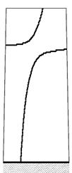
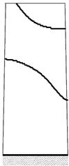
The
vibrations of the compressor blades (Figure 1) are considered. The blades are modeled
by pre-twisted shallow shell with trapezoidal base and variable thickness. The
sketch of the shell base is presented in Figure 2. The shell is clamped on one
side and it is free on others three sides. The coordinate plane (![]() ) passes through the chord of the root section and
the central line of the blade. Moreover, the
) passes through the chord of the root section and
the central line of the blade. Moreover, the ![]() axis
coincides with the central line of the blade. The geometry of the shell middle
surface is complex, therefore, the shell is not considered in principal
coordinates.
axis
coincides with the central line of the blade. The geometry of the shell middle
surface is complex, therefore, the shell is not considered in principal
coordinates.
The
compressor blade previously studied by Meerovich (1956, 1961) is treated. The
shape of the untwisted shell middle surface can be described by the following
function:
 ,
,
where ![]() is the distance between the middle surface and the plane xy in the root section;
is the distance between the middle surface and the plane xy in the root section; ![]() is the length of the root section chord;
is the length of the root section chord; ![]() ;
; ![]() is the distance
between the middle surface and the plane (
is the distance
between the middle surface and the plane (![]() ) on the peripheral
edge;
) on the peripheral
edge; ![]() is the length of the blade. The thickness of the untwisted blade can
be presented in the following analytical form (Meerovich 1961, 1956):
is the length of the blade. The thickness of the untwisted blade can
be presented in the following analytical form (Meerovich 1961, 1956):
 ,
,
where ![]() is the maximal thickness of the root section;
is the maximal thickness of the root section; ![]()
![]() is the maximal
thickness of the peripheral
edge.
is the maximal
thickness of the peripheral
edge.
It
is assumed, that the blade is pre-twisted uniformly and pre-twisted angle is
denoted by ![]() . Then the thickness and the shape of middle
surface can be presented as:
. Then the thickness and the shape of middle
surface can be presented as:
 ;
;
 .
.
The
boundary conditions on the clamped edge are the following:
 , (1)
, (1)
where
![]() ,
,![]() are displacements of the middle
surface points in x, y, z directions,
respectively.
are displacements of the middle
surface points in x, y, z directions,
respectively.
As thin shell is considered, the shear
is not taken into account. Then the potential energy of the shell can be
presented as (Grigoluk, Kabanov, 1978;
Goldenveizer et al. 1979):
 (2)
(2)
where ![]() are the Young’s
modulus and the Poisson’s ratio of the shell material. The parameters of shell deformations
are determined in the following form (Grigoluk,
Kabanov, 1978):
are the Young’s
modulus and the Poisson’s ratio of the shell material. The parameters of shell deformations
are determined in the following form (Grigoluk,
Kabanov, 1978):
![]() ;
; ![]() ;
; ![]() ; (3)
; (3)
![]() ;
;
 ;
;
![]() ;
;
 ;
;
 ;
;
![]() ;
;
 ;
;
 ;
;
![]() ;
;
 ;
;
![]() ,
,
where ![]() are linear components of membrane strains of shell middle surface;
are linear components of membrane strains of shell middle surface; ![]() are components of the bending deformations of the middle surface;
are components of the bending deformations of the middle surface; ![]() and
and
![]() are rotation angles about the tangent vectors to the lines x and y, respectively;
are rotation angles about the tangent vectors to the lines x and y, respectively; ![]() is angle of rotation about normal to the middle surface. Curvatures
of the middle surface are determined as:
is angle of rotation about normal to the middle surface. Curvatures
of the middle surface are determined as:
 ;
;  ;
;  ,
,
where
![]() ,
, ![]()
![]() are coefficients of the first and the second quadratic form of the
middle surface.
are coefficients of the first and the second quadratic form of the
middle surface.
The kinetic energy of the shell has the following form (Amabili, 2008):
 , (4)
, (4)
where ![]() is the shell material density.
is the shell material density.
3. Linear vibrations analysis
In this section the linear vibrations
of the shell are considered and nonlinear terms are not taken into account in the
expressions (3). The Rayleigh-Ritz method is used to determine eigenfrequencies
and eigenmodes of shell, so only the kinematic boundary conditions are taken
into account. The boundary conditions on the shell free edges are natural. Therefore,
they are not taken into account in linear analysis.
The periodic vibrations of the shell are presented in the following
form:
![]()
![]() ;
;
![]()
The
R-function (Rvachev, Sheiko, 1995) is used to satisfy the boundary conditions (1).
R-functions are very useful for shallow shells with complex base analysis (![]() satisfies the
following conditions:
satisfies the
following conditions:
![]()
![]()
![]()
The function ![]() can be derived for
arbitrary domains with analytical boundaries. The methods for these functions construction
are considered by Rvachev, Sheiko (1995).
can be derived for
arbitrary domains with analytical boundaries. The methods for these functions construction
are considered by Rvachev, Sheiko (1995).
According
to the R-function theory, the clamped part of the shell boundary ![]() can be
presented by the following function:
can be
presented by the following function:
![]() ,
,
where ![]() is the
operation of R-conjunction. The functions
is the
operation of R-conjunction. The functions ![]() and
and ![]() describe
describe ![]() axis and
the domain
axis and
the domain ![]() , respectively. These functions can be presented
in the following form:
, respectively. These functions can be presented
in the following form:
![]() ,
, ![]() .
.
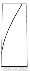
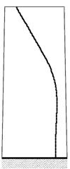
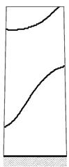
The steps of
the function ![]() construction are shown
in Figure 3.
construction are shown
in Figure 3.
Following
the Rayleigh-Ritz method, the
vibrations modes are presented as:
 ;
;
 ; (5)
; (5)
 ,
,
where ![]() ,
, ![]() ,
, ![]() are trial functions. The expressions (5) satisfy boundary conditions
(1). The following trial functions are used in this paper:
are trial functions. The expressions (5) satisfy boundary conditions
(1). The following trial functions are used in this paper:
 (6)
(6)
where ![]() describes the trapezoidal base of the shallow shell.
describes the trapezoidal base of the shallow shell.
The expressions (5) are substituted into the Lagrange functional ![]() and the integration is carried out. Then the functional
and the integration is carried out. Then the functional ![]() is
obtained as quadratic form of the parameters
is
obtained as quadratic form of the parameters ![]() . In general,
. In general, ![]() can be
presented in the following form:
can be
presented in the following form:
![]() . (7)
. (7)
The
minimum of the Lagrange functional is determined from the following equations: ![]() ;
;![]() . These equations can be presented as the eigenvalue
problem:
. These equations can be presented as the eigenvalue
problem:
![]() (8)
(8)
where ![]() .
.
4. Nonlinear
finite degrees-of-freedom model of vibrations
Nonlinear vibrations of the blade are approximated by the eigenmodes of
linear vibrations. Then the shell bending vibrations ![]() can be
presented as:
can be
presented as:
 , (9)
, (9)
where ![]() are normalized eigenmodes. The displacements
are normalized eigenmodes. The displacements ![]() and
and ![]() are
presented as:
are
presented as:
|
|
(10) |


where ![]() and
and ![]() are eigenmodes of in-plane vibrations. Now the equations (9, 10) are
substituted into the kinetic and potential energy (2, 4) and the integration is
carried out. As a result, the potential and kinetic energies are obtained as
functions of the generalized coordinates and the generalized velocities in the
following form:
are eigenmodes of in-plane vibrations. Now the equations (9, 10) are
substituted into the kinetic and potential energy (2, 4) and the integration is
carried out. As a result, the potential and kinetic energies are obtained as
functions of the generalized coordinates and the generalized velocities in the
following form:

Using
the kinetic and potential energy, the Lagrange equations with respect to the generalized
coordinates ![]() are
derived.
are
derived.
Due to the pre-twist of the shell, the displacements orthogonal to the blade
middle surface consist of both displacements ![]() and
and ![]() . The displacements
. The displacements ![]() have moderate
amplitudes. Therefore, the inertial terms only in the
have moderate
amplitudes. Therefore, the inertial terms only in the ![]() direction are not
taken into account. Then the system of
direction are not
taken into account. Then the system of ![]() ordinary
differential Lagrange equations is transformed into the system of
ordinary
differential Lagrange equations is transformed into the system of ![]() linear
algebraic equations:
linear
algebraic equations:

and the system of ![]() ordinary differential
equations. The solutions of linear algebraic equations are substituted into the
system of
ordinary differential
equations. The solutions of linear algebraic equations are substituted into the
system of ![]() ordinary
differential equations. The following dimensionless variables and parameters
are used in future analysis:
ordinary
differential equations. The following dimensionless variables and parameters
are used in future analysis:
![]() ,
,  ,
,  , (11)
where ![]() is the first (minimal) eigenfrequency. Then the finite degrees-of-freedom
dynamical system with respect to dimensionless generalized coordinates and
parameters has the following form:
is the first (minimal) eigenfrequency. Then the finite degrees-of-freedom
dynamical system with respect to dimensionless generalized coordinates and
parameters has the following form:
 (12)
(12)
where ![]() are known
system parameters. The matrix
are known
system parameters. The matrix ![]() can be presented as
can be presented as
![]()
where ![]() is matrix of dimensionless eigenfrequencies. By means of the
coordinate transformations
is matrix of dimensionless eigenfrequencies. By means of the
coordinate transformations

the system (12) is rewritten with
respect to the modal coordinates:
 (13)
(13)
5. Nonlinear normal modes of vibrations
The
Shaw-Pierre nonlinear normal modes are used to analyze the dynamical system
(13) (Shaw, Pierre, 1993; Jiang et al. 2005; Avramov, 2008;
![]() . (14)
. (14)
Due to these internal resonances, the shell motions have three active generalized
coordinates ![]() . Then the invariant manifold of the system can be presented
as (Jiang et al. 2005):
. Then the invariant manifold of the system can be presented
as (Jiang et al. 2005):
![]() (15)
(15)
This invariant manifold satisfies the
following partial differential equations:

![]() .
.
The
functions ![]() can be
presented as truncated power series as:
can be
presented as truncated power series as:
|
|
(17) |
where ![]() ,
, ![]() ,
, ![]() are unknown
coefficients. As the system (13) is presented with respect to the modal
coordinates, the coefficients of summands (17) with degrees lower than two are
equal to zero (Jiang et al.
2005). The solutions (17) are substituted
into (16) and the summands with
are unknown
coefficients. As the system (13) is presented with respect to the modal
coordinates, the coefficients of summands (17) with degrees lower than two are
equal to zero (Jiang et al.
2005). The solutions (17) are substituted
into (16) and the summands with ![]() are equated. As a
result, the set of the systems of linear algebraic equations is obtained. The
first system is linear with respect to the coefficients of the second degrees (i.e.
the summands with
are equated. As a
result, the set of the systems of linear algebraic equations is obtained. The
first system is linear with respect to the coefficients of the second degrees (i.e.
the summands with  ) and the second system is linear with respect to the
coefficients of the third degrees (i.e. summands with
) and the second system is linear with respect to the
coefficients of the third degrees (i.e. summands with  ). The coefficients of the series (17) are obtained by
solving sequentially these systems of linear algebraic equations. Thus, the
nonlinear mode (15) can be obtained.
). The coefficients of the series (17) are obtained by
solving sequentially these systems of linear algebraic equations. Thus, the
nonlinear mode (15) can be obtained.
The equations (17) are substituted into
the third, fourth and fifth equations of the system (13). As a result, the
system of three ordinary differential equations describing the motions on
nonlinear modes is obtained in the following form:
![]() ,
, ![]() . (18)
. (18)
The harmonic balance method is used to
study the motions on the nonlinear mode (18). The
solutions of the system (18) are presented as:
![]() ,
, ![]() . (19)
. (19)
Substituting
the expressions (19) into the equations (18), the system of nonlinear algebraic
equations with respect to ![]() ;
; ![]() is
derived. This system is solved by the continuation technique (Seydel, 1997).
is
derived. This system is solved by the continuation technique (Seydel, 1997).
To analyze stability of periodic
motions, the system (13) is rewritten in the following vector form:
![]() ,
(20)
,
(20)
where ![]() is phase vector,
is phase vector, ![]() is vector function of
is vector function of ![]() . The stability of periodic motion
. The stability of periodic motion ![]() is analyzed. Following
the book (Yakubovich, Starzhinskii, 1975), small perturbation
is analyzed. Following
the book (Yakubovich, Starzhinskii, 1975), small perturbation ![]() is added to periodic motions. The evolution of small perturbations
in time is described by the following system of ordinary differential
equations:
is added to periodic motions. The evolution of small perturbations
in time is described by the following system of ordinary differential
equations:
![]() (21)
(21)
where ![]() is the Jacobi
matrix.
is the Jacobi
matrix.
Following the book (Parker, Chua, 1989), the fundamental
matrix ![]() of the
system (21) is calculated to analyze stability numerically. This matrix is a
solution of the system (21) with initial conditions in the form of the identity
matrix
of the
system (21) is calculated to analyze stability numerically. This matrix is a
solution of the system (21) with initial conditions in the form of the identity
matrix ![]() . The fundamental matrix at
. The fundamental matrix at ![]() (where
(where ![]() is vibrations period)
is called monodromy matrix (Yakubovich, Starzhinskii, 1975). The conclusions
about the stability of periodic motions are made according to the eigenvalues
of monodromy matrix.
is vibrations period)
is called monodromy matrix (Yakubovich, Starzhinskii, 1975). The conclusions
about the stability of periodic motions are made according to the eigenvalues
of monodromy matrix.
6. Numerical
results
In
order to perform numerical analysis the steel compressor blade is considered with
the following parameters (Meerovich, 1961): ![]() m,
m, ![]() m,
m, ![]() m,
m, ![]() ,
, ![]() m,
m, ![]() ,
, ![]() ,
, ![]() N/m2,
N/m2, ![]() ,
, ![]() kg/m3.
kg/m3.
The calculations
of linear vibrations are carried out by the Rayleigh- Ritz method. The results
of the eigenfrequency calculations are presented in the first row of Table 1. The experimental and numerical data of the previous research, which
are obtained by Meerovich (1961, 1956), are presented in the second and the third
row of Table 1.
Figure
4 shows the nodal lines of the first six eigenmodes ![]() of the blade vibrations. These results are close to the data from (Meerovich,
1961, 1956). However, the eigenfrequency, which is close to the fourth one, is
leaved out in (Meerovich, 1961).
of the blade vibrations. These results are close to the data from (Meerovich,
1961, 1956). However, the eigenfrequency, which is close to the fourth one, is
leaved out in (Meerovich, 1961).
The
first five eigenmodes are used in the expansions (9, 10) to obtain the finite
degrees-of-freedom model of the blade nonlinear vibrations. Excluding the
generalized coordinates ![]() , the system with ten degrees-of-freedom in the form of (13)
is derived. The
, the system with ten degrees-of-freedom in the form of (13)
is derived. The
The
vibrations with dominant generalized coordinate ![]() , which is excited due to the internal resonance (14), are
analyzed. In this case, the generalized coordinate
, which is excited due to the internal resonance (14), are
analyzed. In this case, the generalized coordinate ![]() is close to zero. The
backbone curve of these motions is presented in Figure 5, which shows the
vibrations amplitudes
is close to zero. The
backbone curve of these motions is presented in Figure 5, which shows the
vibrations amplitudes ![]() versus
versus ![]() . The stable and unstable motions are shown on this figure by
solid and dotted lines, respectively. The eigenfrequencies of linear vibrations
are shown by vertical lines in Figure 5. The free vibrations (Figure 5) are
stable until the amplitude of
. The stable and unstable motions are shown on this figure by
solid and dotted lines, respectively. The eigenfrequencies of linear vibrations
are shown by vertical lines in Figure 5. The free vibrations (Figure 5) are
stable until the amplitude of ![]() is small. If the frequency
is small. If the frequency ![]() is increased, the
vibrations amplitude
is increased, the
vibrations amplitude ![]() decrease quickly. Note that the vibrations
decrease quickly. Note that the vibrations ![]() and
and ![]() have the dominant
harmonics with the frequency
have the dominant
harmonics with the frequency ![]() . As follows from Figure 5, the free nonlinear vibrations
become unstable at certain values of the vibration amplitudes. The frequencies
of nonlinear vibrations (Figure 5) are not close to the frequencies of linear
ones. Therefore, the geometrical nonlinearity affects essentially on the shell
vibrations.
. As follows from Figure 5, the free nonlinear vibrations
become unstable at certain values of the vibration amplitudes. The frequencies
of nonlinear vibrations (Figure 5) are not close to the frequencies of linear
ones. Therefore, the geometrical nonlinearity affects essentially on the shell
vibrations.
Now
the vibrations with dominant generalized coordinate ![]() are analyzed. Such
motions are denoted by the number
are analyzed. Such
motions are denoted by the number ![]() on
on ![]() . All motions, which are shown on Figure 6, are unstable.
. All motions, which are shown on Figure 6, are unstable.
Now another type of motions on the nonlinear
mode (15) is considered. In this case the vibrations ![]() have significant
amplitudes; the rest generalized coordinates are not excited. These vibrations
are shown in Figure 7. The free nonlinear vibrations become unstable at some
value of vibrations amplitudes.
have significant
amplitudes; the rest generalized coordinates are not excited. These vibrations
are shown in Figure 7. The free nonlinear vibrations become unstable at some
value of vibrations amplitudes.
The harmonic balance method is used directly
to the system of nonlinear ordinary differential equations (13) to obtain the motions,
which differ from the vibrations on the considered nonlinear normal mode. As a
result, additional type of periodic motions is obtained. The generalized
coordinate ![]() in this regime is active too. These vibrations are shown by the branch
2 on Figure 6. This branch describes the periodic motions, which split off the
motions 1 due to the period doubling bifurcation.
in this regime is active too. These vibrations are shown by the branch
2 on Figure 6. This branch describes the periodic motions, which split off the
motions 1 due to the period doubling bifurcation.
In order to verify the obtained results the direct numerical integration
of the system (13) is carried out. The initial conditions are obtained from the
solution (19). The results are shown in Figure 5 and Figure 7 by dots. The data
of the direct numerical integration are very close to the results of the normal
mode analysis. So, the method suggested in the previous section adequately
describes the system vibrations.
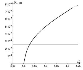
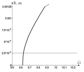
Now the projections of the middle surface points
vibrations on the normal to this surface are treated. The corner points with the
coordinates ![]() and
and ![]() have maximal
displacements. However, the shell in these points is very thin. Therefore, the
displacements of the shell points at small distance from the corner points are
considered. Due to pre-twist of the blade, the displacements in the orthogonal
direction to the middle surface
have maximal
displacements. However, the shell in these points is very thin. Therefore, the
displacements of the shell points at small distance from the corner points are
considered. Due to pre-twist of the blade, the displacements in the orthogonal
direction to the middle surface ![]() contain both
contain both ![]() and
and ![]() . These displacements can be presented as
. These displacements can be presented as
 .
.
The backbone curves are shown in Figure
8, where the vibrations amplitudes  versus
the frequency are plotted. Figure 8 shows the backbone curves of the different
vibration modes. The horizontal line shows the thickness of the shell in the
point, where the vibrations are determined. The motions with dominant generalized
coordinate
versus
the frequency are plotted. Figure 8 shows the backbone curves of the different
vibration modes. The horizontal line shows the thickness of the shell in the
point, where the vibrations are determined. The motions with dominant generalized
coordinate ![]() and with
dominant coordinate
and with
dominant coordinate ![]() are shown
on Figure 8a and Figure 8b, respectively.
are shown
on Figure 8a and Figure 8b, respectively.
7. Conclusions
The compressor blade is described by cantilever, pre-twisted, double
curved, variable thickness shallow shell with trapezoidal base. At the first
phase of the analysis the eigenfrequencies and eigenmodes are determined. The
three internal resonances between the third, the fourth and the fifth
vibrations eigenfrequencies are observed in the system. The different modes of the
compressor blade nonlinear vibrations are described by hard backbone curves. It
is shown that the amplitudes of stable vibrations of peripheral edge are commeasurable
with the blade thickness in this region.
The free nonlinear vibrations become unstable at certain values of the
vibrations amplitudes. Moreover, the frequencies of nonlinear vibrations are
not close to the frequencies of linear ones. Therefore, geometrical
nonlinearity affects essentially on the shell vibrations.
References
Abe, A., Kobayashi, Y., and Yamada, G., 2000. Non-linear
vibration characteristics of clamped laminated shallow shells. J. Sound Vib. 234, 405-426.
Amabili, M., 2008. Nonlinear vibrations and stability of shells and plates.
Avramov, K.V., 2008. Analysis of forced
vibrations by nonlinear modes. Nonlinear
Dyn. 53, 117-127.
Avramov, K.V., Tyshkovets, O., Maksymenko-Sheyko, K.V.,
2010. Nonlinear dynamics of circular plates with cutouts. R-function method.
ASME J. Vib. Acoust. 132, №5, 110-135.
Breslavsky,
Breslavsky, I.D., Strel’nikova, E.A., Avramov, K.V.,
2011. Dynamics of shallow shells with geometrical nonlinearity
interacting with fluid. Comput. Struct. 89, 496-506.
Chen, L.W., Peng, W.K., 1995. Dynamic stability
of rotating blades with geometrical non-linearity. J. Sound Vib. 187, 421-433.
Choi, S.-T., Chou, Y.-T., 2001. Vibration
analysis of elastically supported turbomachinery blades by the modified
differential quadrature method. J.
Sound Vib. 240, 937-953.
Didkovskii, V.N., 1974.
Parametric vibrations of turbomachines in a flow. Strength
Mater. 8, 9-13.
Goldenveizer, A.L., Lidskii, V.B., Tovstik, P.E.,
1979. Free vibrations of thin elastic shells. Nauka,
Grigoluk, E.I., Kabanov,
V.V., 1978. Stability of shells. Nauka,
Hoa, S.V.,
1981. Vibration frequency of a curved blade with weighted edge. J. Sound Vib. 79, 107-119.
Hu, X.X., Tsuiji, T., 1999. Free vibration
analysis of curved and twisted cylindrical thin panels. J. Sound Vib. 219, 63-68.
Jiang, D., Pierre, C., Shaw, S.W., 2005. The
construction of non-linear modes for systems with internal resonance. Int. J. Non-Linear Mech. 40, 729-746.
Liew, K.M., Lim, C.W., 1996. Vibration of
doubly-curved shallow shells, Acta
Mech. 114, 95-119.
Meerovich, I.I., 1956. Vibrations of slightly
curved and pre-twisted blades. Trudy
CIAM 271. Oborongiz,
Meerovich, I.I., 1961. Stress distribution in vibrating compressor blades. Oborongiz,
Mindle, W.L.,
Torvik, P.J., 1987. Multiple modes in the vibration of
cantilevered shells. J. Sound Vib. 115, 289-301.
Mohamed Nabi, S., Ganesan, N., 1996. Comparison of beam and plate
theories for free vibrations of metal matrix composite pre-twisted blades. J. Sound Vib. 189, 149-160.
Pak, C.H.,
Parker T.S., Chua L.O.,
1989. Practical numerical algorithms for chaotic systems.
Pisarenko, G.S., Vorob’ev,
Yu.S., 2000. Issues of simulation of turbomachine blade vibration. Strength
Mater. 32, 487-489.
Ross, C.T.F.,
1975. Free vibration of thin shells. J. Sound Vib. 39, 337-344.
Rvachev, V.L., Sheiko, T.I., 1995. R-function in
boundary value problem in mechanics. Appl. Mech. Rev. 48, 305-316.
Sakiyama, T., Hu, X.X., Matsuda, H., Morita, C.,
2002. Vibration of twisted and curved cylindrical panels with variable
thickness. J. Sound Vib. 254, 481-502.
Seydel, R., 1997. Nonlinear computation. Int. J. Bifurc. Chaos 7, 2105-2126.
Shaw, S.W., Pierre, C.,
1993. Normal modes for nonlinear vibratory systems. J. Sound Vib. 164, 58-124.
Venkatsan, C., Nagaraj, V.T., 1982. Non-linear
flapping vibrations of rotating blades. J.
Sound Vib. 84, 549-556.
Yakubovich, V.A., Starzhinskii, V.M., 1975. Linear Differential Equations with Periodic Coefficients, Wiley,
Fig.
1. Sketch of the blade
Fig. 2. Sketch
of the shell base
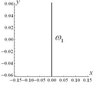
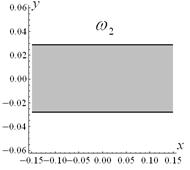
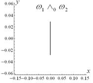
Fig.3.
The steps of the construction of the function ![]() , which describes the clamped part of the shell boundary. The
regions, where the function is positive, are shown by grey color. The black
lines show the zero of the function.
, which describes the clamped part of the shell boundary. The
regions, where the function is positive, are shown by grey color. The black
lines show the zero of the function.

a. b. c. d. e. f.
Fig.4.
The nodal lines of eigenmodes corresponding to the following eigenfrequencies
in Hz:
a.
![]() b.
b. ![]() c.
c. ![]() d.
d. ![]()
e.
![]() f.
f. ![]()
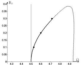
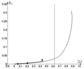
Fig.
5. The backbone curves of the vibrations with dominant
general coordinate ![]()
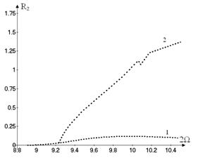
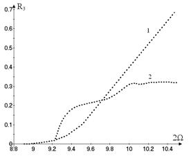
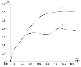
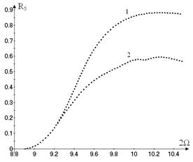
Fig.
6. The backbone curves of the free unstable nonlinear
vibrations
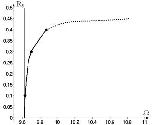
Fig.
7. The vibrations of the shell with dominant general
coordinate ![]()
a.
b.
Fig.8. The
backbone curves of shell vibrations ![]() with dominant general
coordinates: a.
with dominant general
coordinates: a. ![]() ; b.
; b. ![]() .
.
Table
1. Eigenfrequencies of vibrations
|
|
|
Eigenfrequencies
in Hz |
|||||
|
1 |
The results of the calculations |
275.35 |
1020.14 |
1238.08 |
2428.35 |
2628.88 |
3153.8 |
|
2 |
The results of previous calculations (Meerovich,
1961) |
285 |
1000 |
1215 |
2560 |
3280 |
|
|
3 |
The experimental data (Meerovich, 1961) |
273 |
1000 |
1223 |
2457 |
2946 |
|